Enhance a 3-D Chart

1. Click anywhere on the 3-D chart you want to modify.
2. Choose Chart Tools Layout> Background> 3-D View. The Format Chart Area dialog box. The options you see depend on the chart type.
3. From the 3-D Rotation option:
   
   Click the x-axis left or right rotation arrows or enter the degree of left/right rotation (between 0 and 360) you want for the chart in the Rotation box. This rotates the pie slices left or right.
   Click the y-axis up or down rotation arrows or enter the degree of up/down rotation.
   Click the Perspective up or down arrows to change the "camera" view or the view from the top. You can optionally type the elevation angle (between 10 and 80) in the Elevation text box.
   
   
4. From the 3-D Format option:
   
   Choose a Rotation Preset option to select a bevel style for the top or bottom of the chart border.
   Change the thickness of the bars or height of pie slices by entering a value (between 5 and 500) in the Height box.
   Change the Depth option to deepen series bars and the chart floor. This option does not apply to pie charts. Values range from 0 - 2000.
   
   
5. Click Close. The chart appears on-screen, rotated to the angles you selected. A 3-D pie chart before and after changing the elevation and rotation.

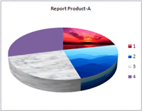
Place a Picture in a Data Series

1. Right-click the series or data point you want to modify. A shortcut menu appears.
2. Choose Format Data Series. The Format Data Series dialog box appears.
3. Click the Fill option. Fill options appear on the right side. Select Picture or Texture Fill.
4. Click File. The Insert Picture dialog box appears.
5. Locate and select the picture you want to use. Click Insert. The Format Data Series dialog box reappears.
6. Click ok. Illustrates a pie chart where three series were replaced one of texture and two with graphic images.