MS-Excel / General Formatting

---

Adjust Chart Data

1. Click anywhere on the chart that you want to modify.
2. Choose Chart Tools Design> Data> Select Data Source. The Select Source Data dialog box opens with the current chart data selected in the worksheet.
3. Click and drag in the worksheet to select the new data range. The Edit Data Source dialog box collapses so you can easily see your data.
4. Release the mouse button. The Edit Data Source box reappears.
5. Click ok. The Edit Data Source dialog box closes.

To quickly add or delete a series to a chart located on the same worksheet as the data, click anywhere on the chart that you want to edit. Notice that Excel surrounds the chart with selection handles and marks the source data in the worksheet with a colored border. Click and drag the corner handle of the worksheet source range to add or subtract cells.

Handling Missing Data or Charting Hidden Data

Sometimes, data that you are charting may be missing one or more data points. Also, by default, Excel does not include data in hidden rows and columns within the data range you're charting. Excel offers several options for handling the missing data and allows you to chart hidden data in a range. Just follow these steps:

1. Click anywhere on the chart and click the Design tab to display the chart design tools on the Ribbon.
2. Click the Select Data button. Excel displays the Select Data Source dialog box.
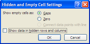
3. Click the Hidden and Empty Cells button. Excel displays the Hidden and Empty Cell Settings dialog box.
4. Select the option that corresponds to how you want to handle the missing data:
   
   
   
   Gaps:
   Excel ignores missing data, and the data series leaves a gap for each missing data point. This is the default setting.
   
   Zero:
   Excel treats missing data as zero.
   
   Connect Data Points with Line:
   Excel calculates missing data by using data on either side of the missing point(s). This option is available only for line charts and some X Y scatter chart subtypes.
   
   
5. If you want to chart hidden data within the chart's source data range, select the Show Data in Hidden Rows and Columns check box.
6. Click OK to exit the Hidden and Empty Cell Settings dialog box, and click OK again to exit the Select Data Source dialog box.

The options that you set apply to the entire active chart; you can't set a different option for different series in the same chart.

Selecting a Chart Element

Modifying an element in a chart is similar to everything else that you do in Excel: First you make a selection - in this case, select a chart element - and then you issue a command to do something with the selection.

You can select a chart element in any of the following three ways:

1. Click the chart element. If the element is a series, clicking the series once selects all the points in the series. Clicking the series twice selects individual points in the series.
2. Press the up-arrow or down-arrow key to cycle through all the elements in the chart. If a data series is selected, you can press the right-arrow or leftarrow key to select individual points in the series.
3. Click the Format tab on the Ribbon and select a chart element from the Chart Elements drop-down list (located above the Format Selection button) in the Current Selection group.

If you move the mouse pointer over a chart element, a ScreenTip displays the name of the element. If the element is a data point, the ScreenTip displays the value. The ScreenTip is useful in ensuring that you're selecting the intended element.

Before you can modify a chart, the chart must be activated. To activate an embedded chart, click it. Doing so activates the chart and also selects the element that you click. To activate a chart on a chart sheet, just click its sheet tab.