MS-Excel / Getting Started

---

Navigating a Spreadsheet

If you have a large spreadsheet, chances are good that information may be hidden by the limitations of your computer screen. To help you view and select cells in different parts of your spreadsheet, Excel offers various ways to navigate a spreadsheet using the mouse and keyboard.

Using the mouse to move around in a spreadsheet

To navigate a spreadsheet with the mouse, you can click the scroll bars or use the scroll wheel on your mouse, if you have one. To use the scroll bars, you have three choices:

• Click the up/down or right/left arrows on the horizontal or vertical scroll bars.
  This moves the spreadsheet one row (up or down) or column (right or left) at a time.
• Drag the scroll box of a scroll bar.
• Click the scroll area (any area to the left/right or above/below the scroll box on the scroll bar).
  This moves the spreadsheet one screen left/right or up/down.

If your mouse has a scroll wheel, you can use this wheel to move through a spreadsheet by two methods:

• Roll the mouse's scroll wheel up or down to scroll your spreadsheet up or down.
• Press the scroll wheel to display a four-way pointing arrow, then move the mouse up, down, right, or left. (When you are done, click the scroll wheel again.)

Using the keyboard to move around a spreadsheet

Using the mouse can be faster to jump from one place in a spreadsheet to another, but sometimes using the mouse can be frustrating, trying to line it up just right. For that reason, you can also use the keyboard to move around a spreadsheet. Some of the common ways to move around a spreadsheet are shown in Table.

Using the Keyboard to Navigate a Spreadsheet

Pressing This	Does This
Up Arrow	Moves up one row
Down Arrow	Moves down one row
Left Arrow	Moves left one column
Right Arrow	Moves right one column
Ctrl + Up Arrow	Jumps up to the top of a column that contains data
Ctrl + Down Arrow	Jumps down to the bottom of a column that contains data
Ctrl + Left Arrow	Jumps to the left of a row that contains data
Ctrl + Right Arrow	Jumps to the right of a row that contains data
Page Up	Moves up one screen
Page Down	Moves down one screen
Ctrl + Page Up	Displays the previous worksheet
Ctrl + Page Down	Displays the next worksheet
Home	Moves to the A column of the current row
Ctrl + Home	Moves to the A1 cell
Ctrl + End	Moves to the bottom right cell of your spreadsheet

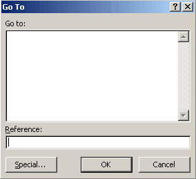
If you know the specific cell you want to move to, you can jump to that cell by using the Go To command. To use the Go To command, follow these steps:

1. Click the Home tab and then click the Find and Select icon in the Editing group. A pull-down menu appears and then click Go To. The Go To dialog box appears. You can also choose the Go To command by pressing Ctrl+G.
   
   
   
   
2. Click in the Reference text box and type the cell you want to move to, such as C13 or F4.
3. Click OK. Excel highlights the cell you typed in Step 2.

Naming Cells

One problem with the Go To command is that most people won't know which cell contains the data they want to find. For example, if you want to view the cell that contains your total amount of money you owe for your income taxes, you probably do not want to memorize that this cell is G68.

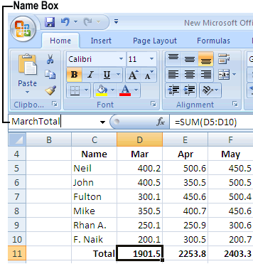
To help you identify certain cells, Excel lets you give them descriptive names. To name a cell or range of cells, follow these steps:

1. Select the cell or cells that you want to name and then click in the Name box, as shown.
   
   
   
   You can type a descriptive name for your cells in the Name box.
   
   
2. Type a descriptive name without any spaces and then press Enter.

After you name a cell, you can jump to it quickly by following this step:

• Click the downward-pointing arrow to the right of the Name box. A list of named cells appears and then click the named cell you want to view. Excel displays your chosen cell.

Eventually, you may want to edit or delete a name for your cells. To delete or edit a name, follow this step:

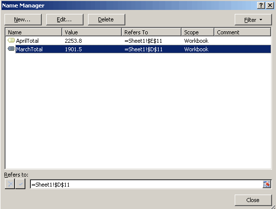
1. Click the Formulas tab and then click the Name Manager icon. The Name Manager dialog box appears.
   
   
   
   
2. Edit or delete the named cell as follows:
   

   To edit the name, click the cell name you want to edit and then click the Edit button. An Edit Name dialog box appears, where you can change the name or the cell reference.
   To delete the name, click the cell name you want to delete and then click the Delete button.

3. Click Close.