Formatting Numbers and Labels
When you first create a spreadsheet, numbers and labels appear as plain text. Plain labels might look boring, but plain numbers (such as 8495 or 0.39) can be difficult to read and understand if the numbers are supposed to represent currency amounts ($8,495) or percentages (39%).
To make labels visually interesting and numbers appear more descriptive of what they actually represent, you need to format your data after you type it into a spreadsheet.
You can format a cell or range of cells after you have already typed in data or before you type in any data. If you format cells before typing any data, any data you type in will appear in your chosen format.
Formatting numbers
To format the appearance of numbers, follow these steps:
- Select one or more cells using the mouse or keyboard. To select multiple cells, drag the mouse or hold the Shift key while pressing the arrow keys.
- Click the Home tab and then click the Number Format list box in the Number group. A pull-down menu appears.
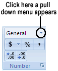
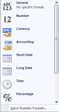
The Number Format list box lists the different ways you can format the appearance of numbers.
The Number group also displays three icons that let you format numbers as Currency, Percentage, or with Commas in one click, as shown in Figure. If you click the downward-pointing arrow to the right of the Accounting Number Format icon, you can choose different currency symbols to use such as $, £, or €.
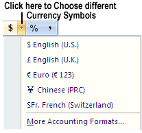
- Click a number format style, such as Percentage or Scientific. Excel displays your numbers in your chosen format.
Displaying negative numbers
Because many people use spreadsheets for business, they often want negative numbers to appear highlighted so they can see them easier. Excel can display negative numbers in parentheses (-23) or in red so you cannot miss them. To define how negative numbers appear in your spreadsheet, follow these steps:
- Select the cell or range of cells that you want to modify and then click the Home tab.
- Click the Format icon in the Cells group. A pop-up menu appears.
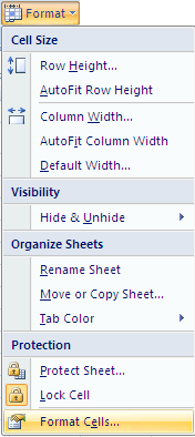
The Format icon lets you format the appearance of rows, columns, or individual cells. - Choose Cells. The Format Cells dialog box appears.
- Choose Currency or Number from the Category list.
You can choose how to format negative numbers only if you format your numbers using the Currency or Number category. - Click a negative number format and then click OK. If any of your numbers become negative in the cell or cells you selected
in Step 1, Excel automatically displays those negative numbers in the negative number format you chose.
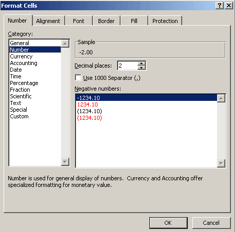
The Format Cells dialog box lets you customize the appearance of your numbers.
Formatting decimal numbers
If you format cells to display numbers with decimal places, such as 23.09 or 23.09185, you can modify how many decimal places appear. To define the number of decimal places, follow these steps:
- Select the cell or cells that contain the numbers you want to format and then click the Home tab.
- Click in the Number Format list box and choose a format that displays decimal places, such as Number or Percentage. Excel formats the numbers in your chosen cells.
You can click the Increase Decimal (increases the number of decimal places displayed) or Decrease Decimal icon (decreases the number of decimal places displayed).
