MS-Excel / General Formatting

---

Filtering Data in a Table

Filtering data is one of the most common activities performed with a table. Often, you want to view or analyze a subset of the data in a large dataset. When Excel creates a table, it includes a sort and filter drop-down arrow to the right of each column header. After you filter your table, the status bar displays the number of rows visible.

You can use Excel's filtering features in a standard (non-table) range. Select the range, click the Sort & Filter button on the Ribbon's home tab, and choose Filter from the menu to add the sort and filter drop-down arrows to the header row. A worksheet can have only one sort and filter range but can have many tables, each with its own sort and filter settings.

If your table data was imported from an external range, your table filters and sort orders are normally reapplied after you refresh the range (import the latest data). If you add data rows manually, however, you must click the Sort & Filter button in the Ribbon's Home tab and then choose Reapply from the menu before Excel will update the table.

Filtering based on individual column entries

Follow these steps to filter your table data based on the individual entries in a column:

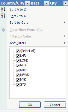
1. Click the arrow on the header of the column you want to filter. Excel displays the Sort and Filter menu.
   
   
2. The lower portion of the menu displays the unique column entries in a window. By default, Excel selects all entries. If you want to display rows for one or only a few entries, clear the Select All check box and individually select the items you want displayed. Alternatively, if you want to hide rows for only a few entries, clear the check boxes next to these entries but do not clear the Select All check box.
   The ability to select multiple column entries is new in Excel 2007. Also, the list can display up to 10,000 unique entries (compared with 1000 entries in earlier versions of Excel).
3. Click OK. In the table, Excel displays rows for all the entries you selected in Step 2 and hides all rows for the cleared entries. If your table uses an alternative row-banding style, the banding is preserved after you filter table rows. Excel also adds a filter icon (a small funnel) on the column drop-down to indicate that a filter is applied to the column.
4. To filter additional columns, repeat Steps 2 and 3.

If your column has a series of date entries (month, day, year), Excel allows you to filter at the year, month, or day levels. In the column items list window, only the year level is listed initially. If you click the plus sign (+) next to a year, the months for that year are listed. Clicking the plus sign next to the month displays individual day entries for that month.

Filtering based on column data type

Suppose you have a table column that contain dates. But instead of filtering the column based on individual dates, you want to display dates for the current month, last month, last quarter, or year to date. Or suppose you have a numeric column and want to display records exceeding a certain value or lying between two values. Or perhaps you have a text column and you want to display records that begin with certain text or contain certain text. Excel 2007 provides many filtering options that you can apply based on the type of data you have in a column.

To filter a table data based on date, number, or text criteria, follow these steps:

1. Click the arrow on the header of the column you want to filter. Excel displays the filter and sort menu.
2. Immediately above the window that displays individual column entries, choose the datatype Filters option (where datatype is Text, Number, or Date, depending on the data type of the column you are filtering).
3. Choose a specific filter option from the flyout menu or choose Custom Filter at the bottom of the menu to display a dialog box that offers additional options.
4. If your choice in Step 3 displays a dialog box, complete the dialog box options and click OK.

Filtering based on cell color

Excel 2007 allows you to filter by cell color. Colors are cell background or font colors applied manually or by conditional formatting. Colors can also include color scales and icon sets.

You can filter by only one color at a time.

To filter your table data based on color formatting, follow these steps:

1. Click the arrow on the header of the column with the color formatting you want to filter. Excel displays the Sort and Filter menu.
2. Choose Filter by Color, and then choose a color option from the flyout menu. You can also choose the No Fill option to filter out all cells with font or background formatting.

Colors for filtering do not include colors defined in the table style, so your table formatting is preserved after color filtering.